Sensitivity Analysis
Updated 2018-07-22
Sensitivity Analysis
Sensitivity Analysis is when we look at the change in output given some change in input. Similar to derivatives if you will (\(\frac{\Delta y}{\Delta x}\)). It is said to be sensitive if the output changes a lot with a small input.
The two types of sensitive analysises are break-even analysis and what-if analysis.
Break-Even Analysis
How much do we adjust our inputs such that our NPV or rate or return break-even
Break-even analysis is typically represented as a break-even chart that indicates clearly where two alternatives equal to each other.
Example: staged construction
We have two options (assuming 8% interest rate):
- Construct full-capacity building now for $140k
- Two stages: construct first stage now for $100k and second stage at time \(n\) for $120k
Notice that if we choose option 2 with \(n=0\), then the present worth of cost is $220k, not worth it compare to option 1.
However if we change the input \(n\) to a further date such that the cost discounted to present worth is less, then the present worth of cost of option 2 decreases:
\(n\) \((P/F, 8\%, n)\) PW of cost 5 0.6806 $182k 10 0.4632 $156k 15 0.3333 $140k 20 0.2145 $126k 30 0.0994 $112k We see that the option 2 breaks-even with option 1 if we decide to construct the second stage at \(n=15\). Any \(n\) beyond that, we should choose option 2 over option 1.
Plotting \(n\) on the x-axis, we can see break-even point graphically:
<img src=”assets/image-20180722155806991.png” width=40%>
What-If Analysis
What if the revenue decreases by 5%, or what if cost to X increases by 12%, etc. How will the output change.
The what-if analysis shows how much a parameter must change to alter an economic decision and assess the inherent risk in a project. This is easily done in a spreadsheet by altering the variables.
Example:
Suppose the following base case: initial cost $300k, annual benefit $85k, salvage value $60k, lifetime of 6 years, and MARR of 14%.
The base case uses the standard, unmodified numbers for cost, benefits, lifetime, interest, etc.
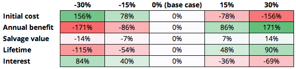
Then we can set a few scenarios and setup a matrix where each base case property is increased or decreased by some percentage (in particular, -30%, -15%, +15%, and +30%). The modified values are in the table below.
-30% -15% 0% (base case) 15% 30% Initial cost $210,000 $255,000 $300,000 $345,000 $390,000 Annual benefit $59,500 $72,250 $85,000 $97,750 $110,500 Salvage value $42,000 $51,000 $60,000 $69,000 $78,000 Lifetime 4.20 5.10 6.00 6.90 7.80 Interest 10% 12% 14% 16% 18% Then we can comptue the NPV for each of the modified parameters. Note that each NPV is assuming only one parameter is changing at a time.
-30% -15% 0% (base case) 15% 30% Initial cost $147,872 $102,872 $57,872 $12,872 $(32,128) Annual benefit $(41,289) $8,291 $57,872 $107,452 $157,033 Salvage value $49,671 $53,772 $57,872 $61,972 $ 66,072 Lifetime $(8,431) $26,673 $57,872 $85,600 $110,244 Interest $106,617 $81,023 $57,872 $36,874 $17,779 We can notice how sensitive the NPV was to which input once we found the difference and color code the change.
We see that initial cost and annual benefit changes the output the most, therefore they’re the most sensitive variables.
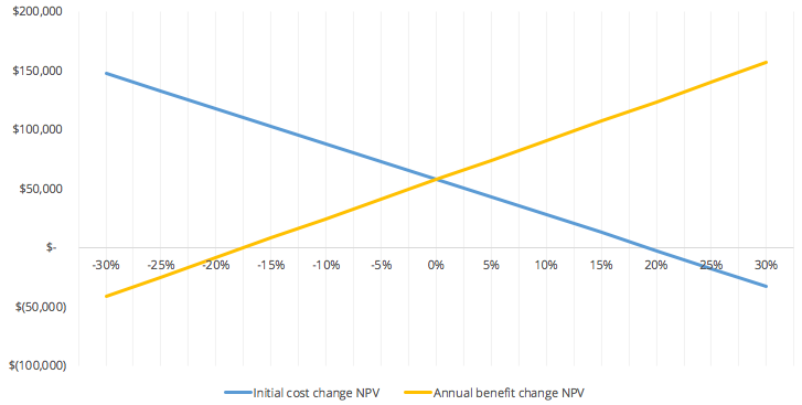
We can also do a break-even analysis for the two sensitive variables, initial cost and annual benefit, to see at which point the output, NPV is $0.
For initial cost, the break even point is at approximately +20% of the base case. For annual benefit, the break even point is at approximately -17.5% of the base case.